Maintenance Cost
Maintenance cost is the regular expense an agency bears to keep an asset on its life cycle path. If no maintenance is carried out, assets will deteriorate at a faster rate than their life cycle path of progression. For example, regular patching up of potholes on a sealed road is road maintenance work. While this does not increase the service potential of the road it helps to prevent rapid deterioration of the road condition. Maintenance cost is closely related to the physical condition of the asset as well as other service criteria such as functionality and capacity. As asset condition deteriorates the asset requires more maintenance, which means an increase in maintenance cost.
Predictor's powerful maintenance module allows the factoring in of future maintenance costs which depend on how well or poorly the asset stock performance is predicted to be over the asset life cycle. To help calibrate the unit costs it simulates current maintenance funding, which can then be compared with actual maintenance funding.
Predictor models the maintenance funding requirements of an individual asset based on asset service conditions such as physical condition, functionality, capacity of the asset, obsolescence. A User-applied maintenance unit cost (maintenance cost needed for a unit network measurement) is applied for each service condition score to reflect the service condition of an asset depending on where it sits on its life path. Users can define the maintenance treatment unit costs relative to each service criteria or the overall condition index.
Maintenance Configuration
The maintenance configuration in Assetic Predictor is typically undertaken by utilizing the organization’s current annual maintenance spend on the asset stock being modeled and then applying unit rates either evenly among a number of condition states for each service criteria or apportioning the unit rate for each service criteria by applying a percentage of the total maintenance budget based on internal logic, knowledge or experience.
The following examples illustrate these two such methods with regards to configuring the maintenance rates utilizing historical maintenance expenditure profiles.
The first step is to identify the actual current network measure for each condition state, by generating a pie chart within the transformed data area of your data.
- Select Show Pie Chart
- Select the service criteria from the drop down and ensure that the network measure radial is selected
- Right click now and select show labels and resolve overlapping, then select display labels as absolute
The result should provide you with a pie chart as per that below. Repeat for all other service criteria.
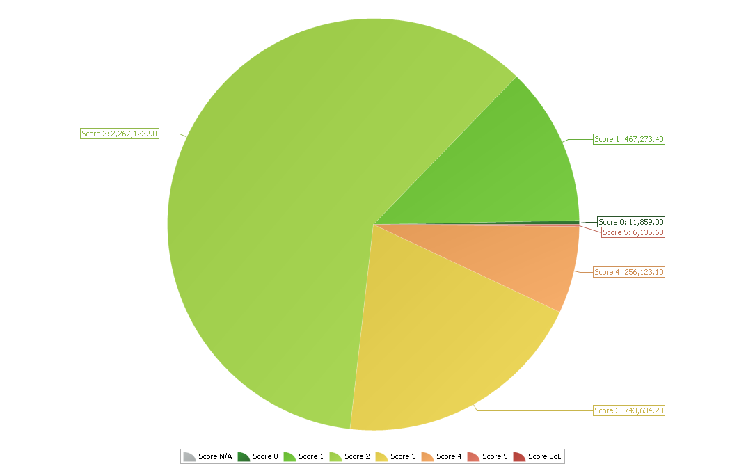
In this example Template we are using two Service Criteria, Pavement Condition Index (PCI) and Surface Condition Index (SCI).
The results of the existing asset stock distribution in this example, by network area and corresponding condition is as follows:
| Condition States | 0 | 1 | 2 | 3 | 4 | 5 | EoL | Total Network Measure (m2) | |
| Service Criteria | SCI | 11,859.00 | 467,273.40 | 2,267,122.90 | 743,634.20 | 256,123.10 | 6,135.60 | - | 3,752,148.20 |
| PCI | - | 2,105,146.70 | 1,406,661.00 | 177,239.80 | 63,100.70 | - | - | 3,752,148.20 |
Method 1 – Even Unit Rate Distribution
- Existing or last year’s maintenance budget is $900,000 with $300,000 allocated to rectify surface defects and $600,000 allocated to rectify pavement defects.
- Decide which condition states on average are deemed appropriate for such maintenance activities to occur.
- In this example it is assumed from local knowledge and experience that these maintenance funds are typically spent when the roads are in condition 2 or worse. Alternatively if you have a maintenance management system that collects this information, you can obtain real actual data from this system.
- The sum of SCI network measure in condition states 2 or worse is 3,273,015.8m2. Divide $300,000 by this sum which equates to $0.092.
- Repeat this step for the second service criteria in this case being the PCI. The sum of PCI network measure in condition states 2 or worse is 1,647,001.5m2. Divide $600,000 by this sum which equates to $0.364.
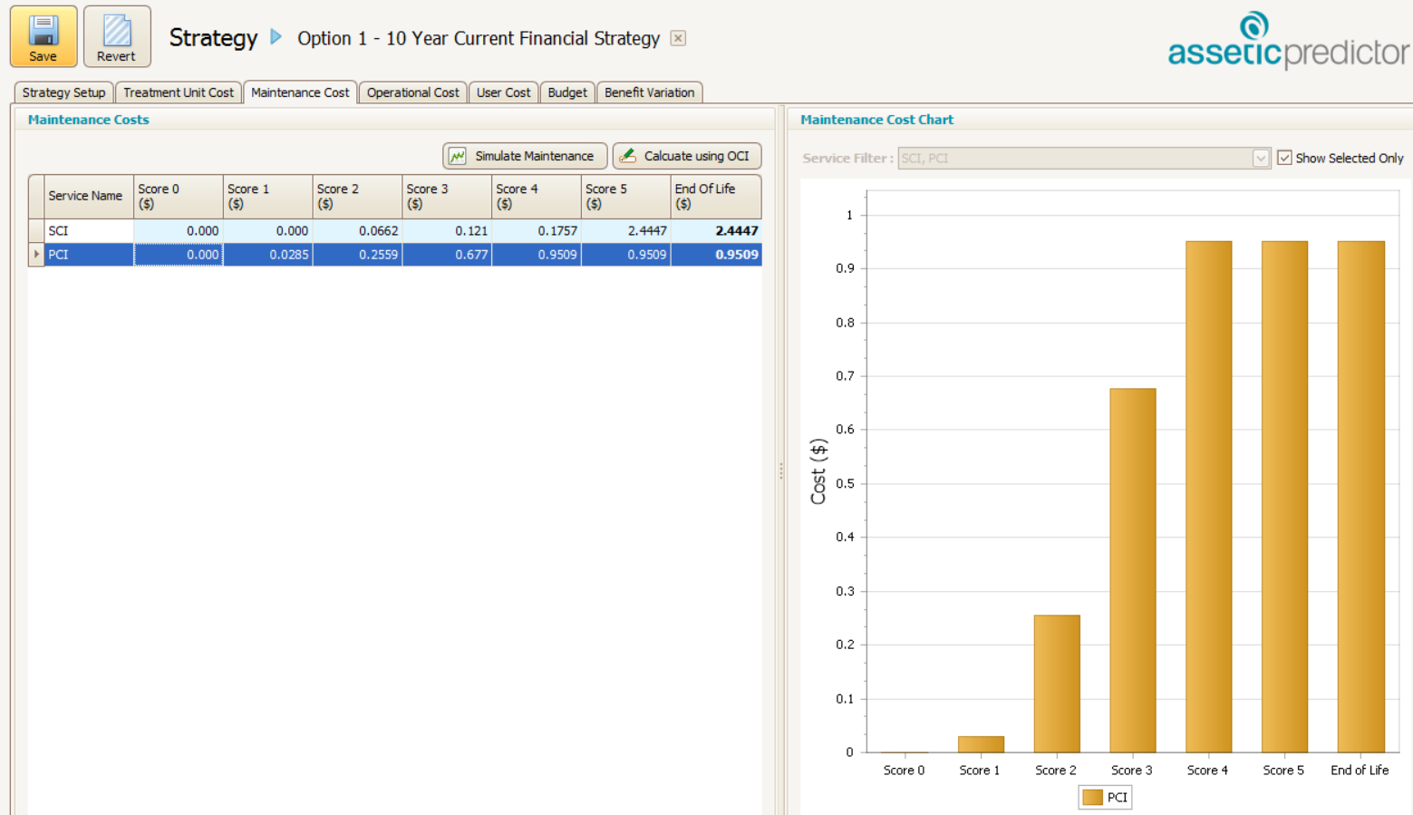
- Apply these rates to the corresponding cells in the maintenance cost tab of your strategy as per the below example.
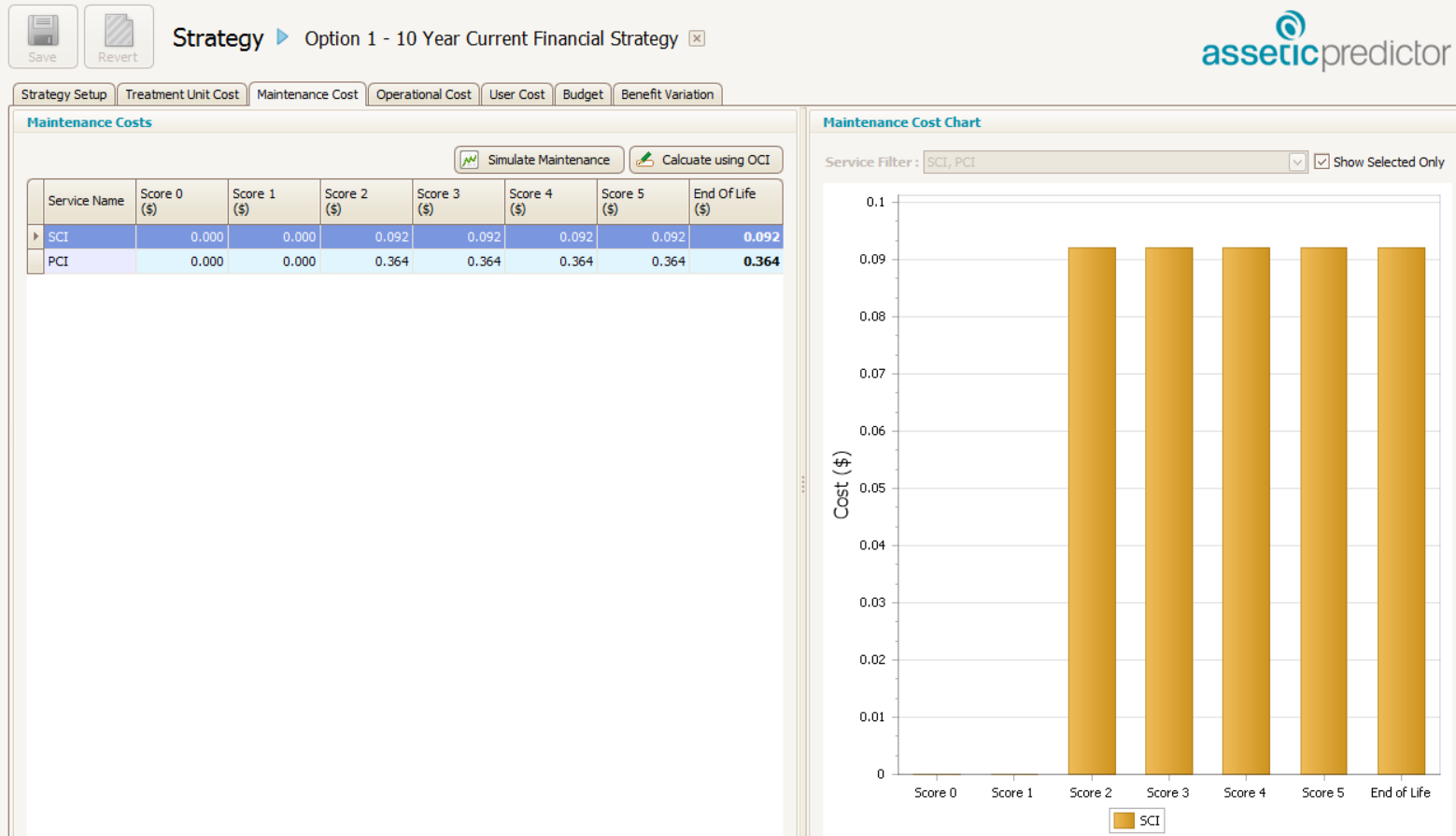
The unit values which have been populated into these cells when multiplied by the asset stock network measure, will return the annual maintenance spend of $900,000. To confirm that this is the case, select the simulate maintenance button and then the corresponding dataset from which you have generated the network measure distribution table. Select run simulation.
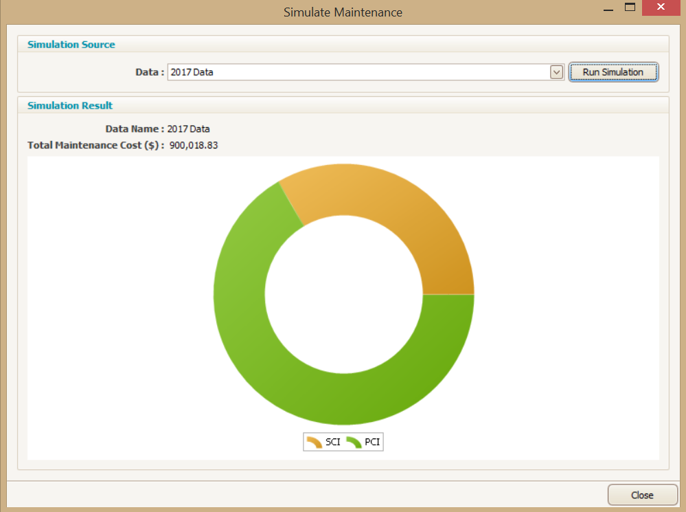
The following chart is generated by Predictor.
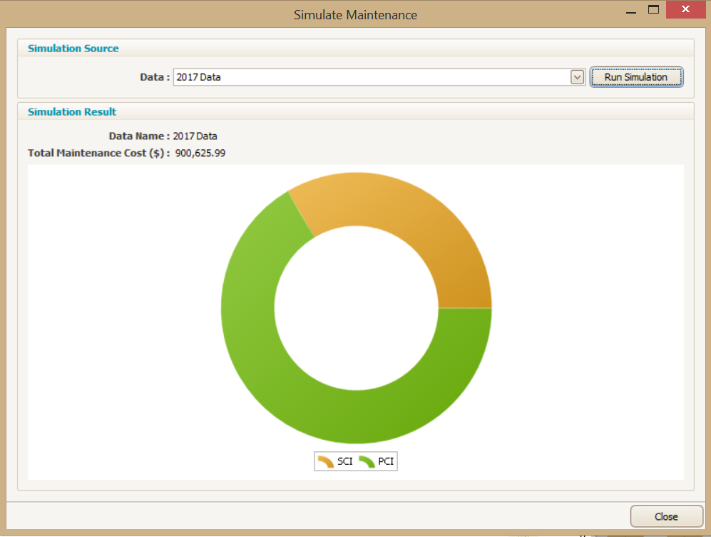
As you will notice in this example, the returned maintenance allocation is calculated at just a little over $900,000, accounting for rounding such a large dataset.
Method 2 – Percentage Apportionment Distribution
- Download the Excel ‘Maintenance Costs Calculations Template’
- Existing or last year’s maintenance budget is $900,000 with $300,000 allocated to rectify surface defects and $600,000 allocated to rectify pavement defects
- Enter the maintenance budget in cells A19 and H19
- Populate the network measure per each condition state
- Decide which condition states on average are deemed appropriate for such maintenance activities to occur.
- In this example it is assumed again from local knowledge and experience that these maintenance funds are typically spent when the roads are in condition 2 or worse. However, information from our maintenance management system and/or finance system has allowed us to identify the distribution of funds per each condition state.
- Populate the % budget allocation for columns C and J.
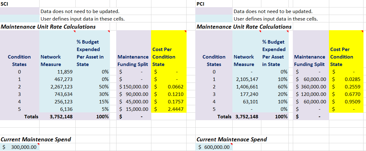
8. Apply these rates from columns F and M, to the corresponding cells in the maintenance cost tab of your strategy as per the below example.
The unit values which have been populated into these cells when multiplied by the asset stock network measure, will return the annual maintenance spend of $900,000. To confirm that this is the case, select the simulate maintenance button and then the corresponding dataset from which you have generated the network measure distribution table. Select run simulation.
The following chart is generated by Predictor.
Predictor is now configured to calculate and determine the future maintenance requirements of your asset portfolio, as a result of various capital works financial strategies, taking into account the predicted asset portfolio changes.